Differentiable phase-space simulation of irradiance
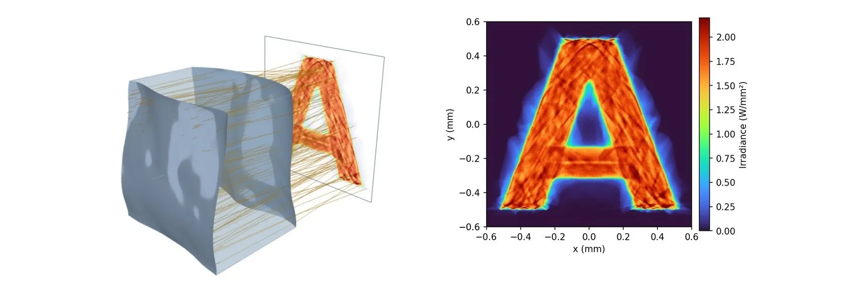
In April 2026, I had the opportunity to visit Strasbourg, France for the Illumination Optics Conference, part of SPIE Optical Systems Design. I presented a fun concept I have been exploring for differentiable simulation and optimization of illumination systems, based on a phase-space representation of the optics.
Below are slides and notes from the presentation. If you or your university has a subscription to SPIE Digital Library, you can also view a recording at https://doi.org/10.1117/12.3098675.

Associate Professor, NTNU Department of Mechanical and Industrial Engineering
This was the last talk of the last session of the day, so I tried to make it somewhat fun and visual. I usually work more on the solar concentration side of nonimaging optics, but this concept is illumination-oriented.
The overall goal of what we are doing here is to design optical systems through optimization: Simulate an optical system, compare the behavior of the system to some kind of objective, and adjust the system until the behavior has the properties we want. In this case the behavior we are looking for is a certain irradiance on some target surface, and the focus of this talk will be on the simulation part itself. We need a fast, smooth, and differentiable simulation method to make this work.
Light Source
Nonimaging Optics Design Competition 2025
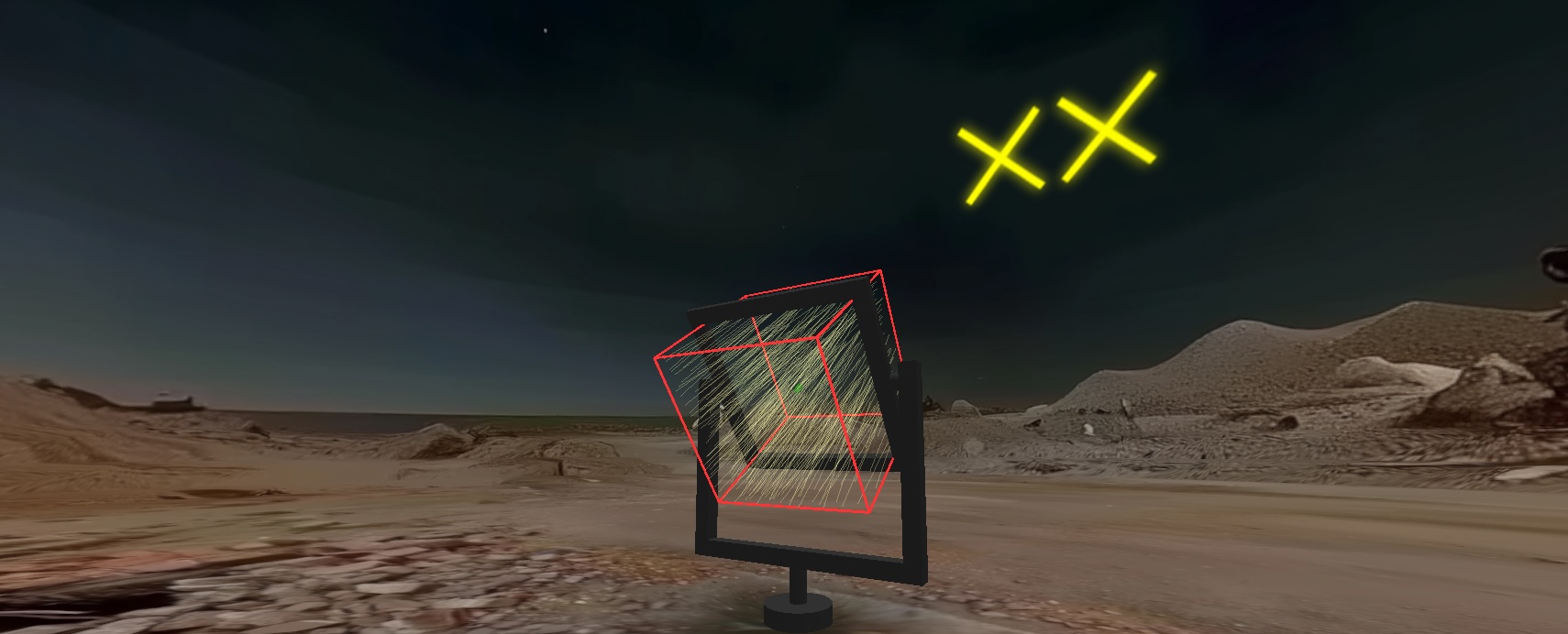
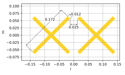
I will present our concept by looking at an example optical system. This means that we need a light source, and I decided to go for a fun one: the XX-shaped sun from the 2025 nonimaging optics design competition. This was a competition we organized as part of the Nonimaging Optics Conference, and the goal was to design an optical system to focus the light from this XX-shaped sun down to a small rod. For now, we will just use this source as an example of some non-trivial light source to simulate through an optical system.
Light source
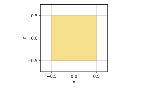
Uniform spatial distribution
XX-shaped angular distribution
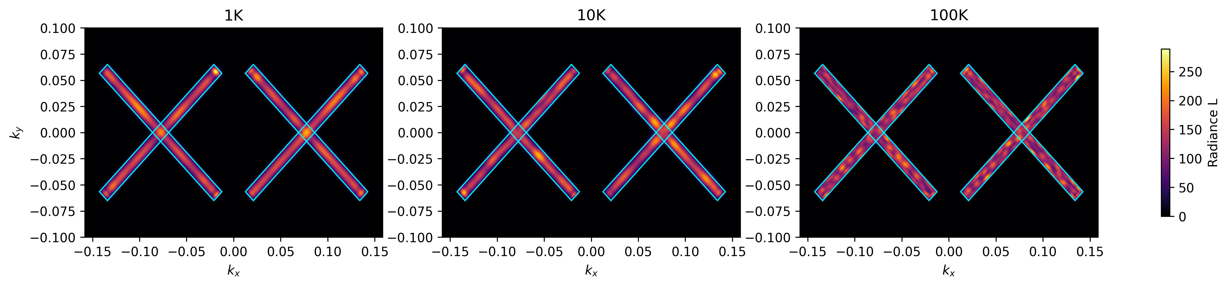
This source is uniform spatially, and XX-shaped in direction-cosine space. So the question is now: How do we simulate some optical system where the light comes from this light source?
As an example, we simulate a pair of freeform lens surfaces in front of a target surface. The question we want to simulate is: What is the irradiance distribution on this target surface?
Simulate irradiance distribution
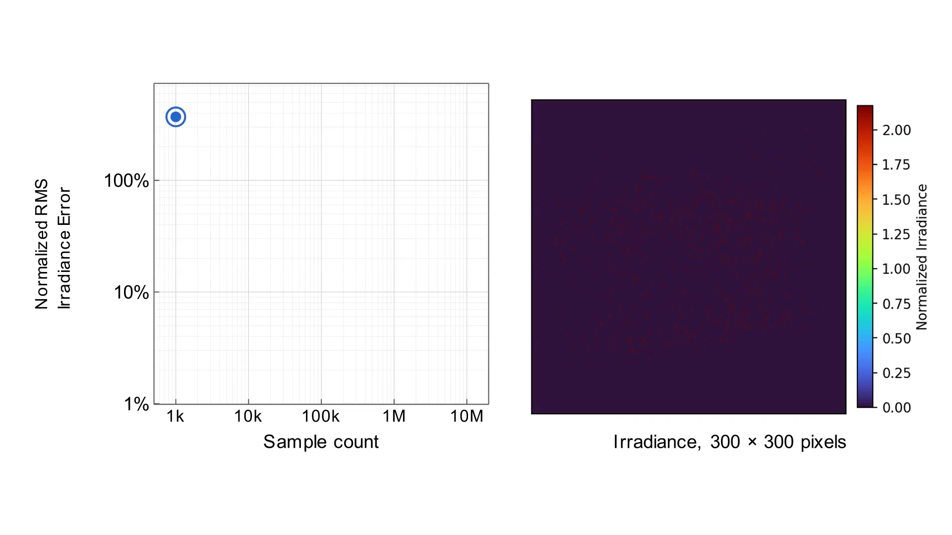
The classical way to simulate this is to divide the target surface into a grid of pixels, trace a bunch of rays through the optical system, and distribute their energy to the pixel it strikes. The result is very noisy, but once we trace enough rays we get a clear picture of the irradiance on the target surface.
When you choose a large number of rays, you see that the irradiance distribution actually consists of different XX-shaped images of the source in different parts of the target surface, due to focusing of the light by the random freeform surface profiles.
We also see that the simulation error falls nicely with , where is the number of rays traced. This looks like a straight line in the log-log-plot and is the classical Monte Carlo convergence behavior.
A sneak peek at the new method
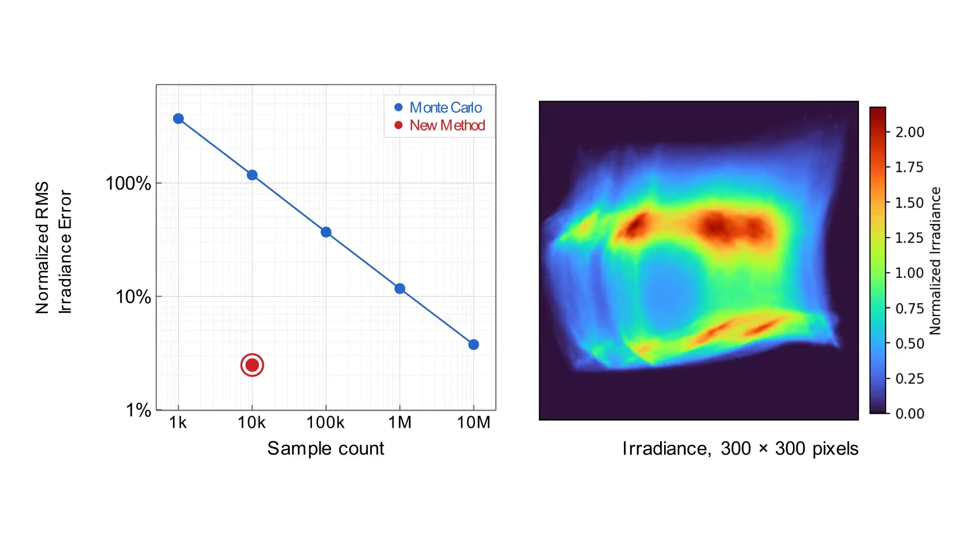
Our goal is to simulate this irradiance distribution, but with smaller error and smaller number of rays. Above is a sneak peek showing that this is going to be possible: We can run a simulation with 10k rays and get an error lower than what we got with 10M rays originally. Let’s figure out how this works by first considering a simpler 2D case:
Here we have a 2D optical system (left side plot) where light comes from a planar source, propagates through a double-sided freeform lens, and ends on a planar target. The fact that the system is 2D makes it possible to visualize the propagation of light through the system from a phase space perspective (right side plot).
In phase space, we plot the position and direction of the light in our system as it crosses some reference surface. On the horizontal axis we have the physical position of the light on the reference surface, and on the vertical axis we have the direction of the light on the reference surface.
Now we can see what happens to the light through the optical system: Each time the light crosses a lens surface, the light is sheared vertically in phase space (the light changes direction), while each time light propagates forwards it is sheared horizontally (the light changes position).
When we look at the optical system from the phase space perspective, it looks very well-behaved. The light is sheared and stretched, but it is still a continuous distribution in phase space.
Assuming the source has constant radiance, there is an easy way to use this phase space distribution to calculate irradiance: The irradiance at any point is the height of the phase-space distribution at that point.
This leads us to the method shown above, which works very well for simple 2D optical systems, and as a visualization tool for understanding why a certain optical system produces a certain irradiance distribution.
The goal is now to extend this method to more complex optical systems, where radiance may not be constant, there may be discontinuities in the optics that make the phase space distribution discontinuous, and the system is 3D instead of 2D?
Instead of looking at the full region in phase space, we can look at a tiny patch of phase space. This is like a “fat ray”, a ray that carries its position but also a certain spatial and angular extent.
Locally, the transformation is mostly smooth even if the full optical system creates discontinuities in phase space. We can use this local smoothness to trace a region in phase space instead of just an infinitesimal ray, like a Taylor expansion. We can trace a small patch of phase space: the patch centre is propagated through the optical as normal, while its shape is transformed by the Jacobian of the transformation.
A round input patch can therefore become an ellipse at the target, and we therefore know exactly the irradiance contribution of this patch at the target surface. Depending on the local geometry of the transformation, it will sometimes be stretched into a wide and flat ellipse, creating a wide and low irradiance contribution. Other times it will be compressed into a tall and narrow ellipse, creating a high and narrow irradiance contribution.
If we fill our input phase space with many of these patches, we can propagate them through the optical system and sum their contributions to get the total irradiance distribution on the target surface as illustrated above. This is close to the core of our method, but we still need to do some tweaks until we are ready for simulating full 3D optical systems.
Real optical systems are three-dimensional, and the corresponding phase space is four-dimensional (when light crosses a surface it has two position components and two direction components). Packing spheres in 2D is already hard, and packing spheres in 4D is even harder leading to either gaps between the spheres or overlaps between the spheres.
Additionally, we have currently assumed that all input patches have the same shape, but this may not be ideal. Close to the edge of a source we may for instance want to compress the input patch to avoid sampling outside the source, and in other parts of the source we may want to stretch the input patch to cover more area. We therefore need a more flexible way to fill phase space with patches.
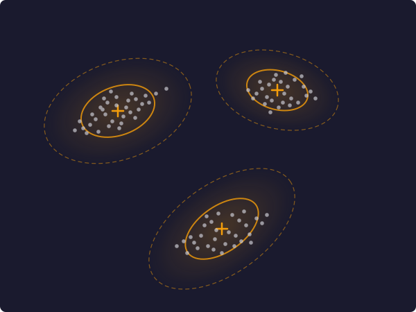
Instead of packing circles, we can fit many elliptically shaped Gaussian distributions to the input phase space and propagate those Gaussians to the target surface.
This has the very nice property that integrating out the directional components of a Gaussian is equivalent to just dropping those components. So it becomes very easy to calculate the irradiance contribution of a Gaussian at the target surface.
This is the approach. The remaining question now is how to actually implement this efficiently.
Using established algorithms
Gaussian Splatting
Kerbl et al., SIGGRAPH 2023
Expectation-maximization Gaussian Mixture Model
Dempster, Laird & Rubin, JRSS 1977
It turns out that we are helped by some well-established algorithms.
Our first job is to represent our input phase space as a set of Gaussian distributions. This is exactly what the Expectation-Maximization algorithm does when fitting a Gaussian Mixture Model to some data.
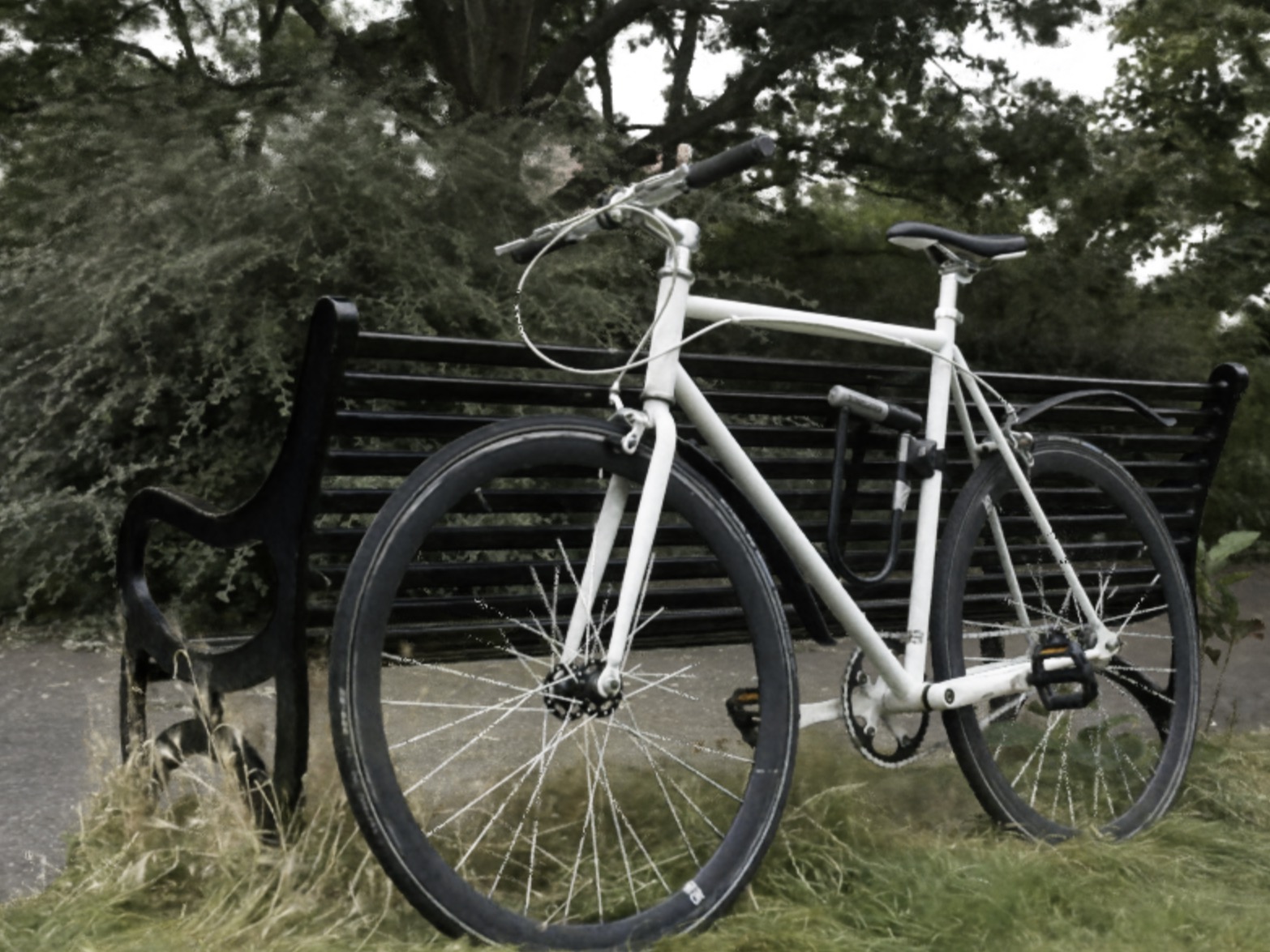
Our second job is to rasterize the final Gaussians to generate the resulting irradiance distribution. Here we can look to Gaussian Splatting, a fairly new concept from 2023 for 3D reconstruction. It is not exactly the same as what we are doing, but part of implementing Gaussian Splatting is to rasterize a bunch of Gaussians in a fast and differentiable way on a GPU, which is exactly what we need to do. We can therefore use rasterization kernels inspired by those used in Gaussian Splatting, but simplified for our case where the Gaussians do not need to be sorted and they combine additively.
We are now ready to simulate a real optical system. The approach is summarized above: The preparation step fits a Gaussian Mixture Model to a set of rays sampled from the source. This set of rays can be anything, e.g. a ray-file supplied by a LED manufacturer, or any other set of rays. We don’t depend on the source having uniform radiance or having a certain shape, as long as we can sample rays from it. This is somewhat expensive but only needs to be done once per source.
After the preparation step, each simulation step consists of tracing the Gaussian centers through the optical system. But instead of tracing only the rays, we also trace their Jacobians (this can be done with automatic differentiation and is equivalent to differential ray tracing or tracing “fat rays”). We then transform the covariances of our Gaussians by the local Jacobian, project them to 2D, and rasterize the resulting Gaussians on the target surface. That’s it. This is fast and differentiable, and can be used in an optimization loop to design optical systems.
There are some additional details to get this to really work. For the Gaussian Mixture Model fit, we need to add some regularization. We depend on the local linearity of a phase space transformation, so we need to make sure that the sampled Gaussians are small enough that this holds to some extent. We also need to make sure that the kernels have large enough footprints that they don’t fall between pixels on the target surface (or we can subsample each pixel if we want to reduce the need for this).
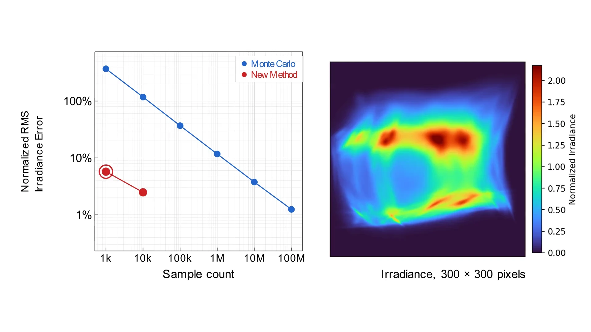
With this, we have an approach that seems to work. Above is simulated irradiance distributions and error at different ray counts, and we see that we need something like three orders of magnitude fewer rays to get the same error as the classical Monte Carlo approach.
This comparison is not completely fair: The classical Monte Carlo approach is naive, and it can be improved with some amount of smoothing, low-discrepancy sampling, and other tricks. Additionally, each ray that we trace in our method is more expensive than a ray in the classical Monte Carlo approach, by approximately a factor of 3-5. Still, the fact that we can get the same error with three orders of magnitude fewer rays is very promising.
An interesting next question is whether we can use this method to design optical systems.
As a quick test, we set up a problem where the goal is to design magic windows that produce letter shapes on a target surface when illuminated by the XX-shaped sun.
The strange source shape and the high contrast ratio between the letters and the background makes this problem challenging with classical tailoring methods, so we fired up some Modal cloud GPUs and designed a few lenses, capping the optimization time to 10 minutes per letter.
Results: Letter A
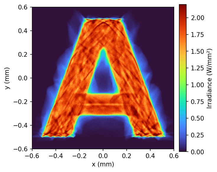
The approach seems to work. We clearly generate the desired letter shapes on the target surface, and the optimization converges nicely. There is still some high-frequency XX-like structure in the illuminated region and some bleeding into the dark region, but overall the approach seems to work well.
A couple of words on the objective function that we used. This can be quite fast because everything runs on the GPU. So like 15 milliseconds for 10,000 or 28 milliseconds for 100,000 rays. But the most important is this lower line forward plus gradient. So we have 603 parameters, and we can use reverse-mode automatic differentiation to get all of these gradients in a single backward pass (unlike the 600x computational cost if we used finite differences like conventional optical design software).
Limitations
- Sharp radiance boundaries become smooth
- Harder to estimate convergence
Gaussian Mixture Model fitting is somewhat expensive (10M Gaussians, approx 10 minutes on a GPU)
There are still some challenges with this approach. One challenge is that many real-world light sources have sharp edges, while the Gaussian Mixture Model fitting will smooth these edges out to some extent. Estimating convergence is also harder. In conventional Monte Carlo simulation, you have a lot of noise but at least the error is predictable. Here, you don’t really know. And the amount of error becomes a trade-off between bias and variance depending on the size of your Gaussians, similar to the bias-variance trade-off in kernel density estimation which this approach shares many similarities with.
As a final shameless plug, you’re all welcome to check out the design challenges that we run as part of the Nonimaging Optics Conference.
Are you interested in exploring this method further? Feel free to reach out to me to discuss potential improvements and possible ways to work together on this.